What are Popular Types of Neural Networks
Types of artificial neural networks.
There are many types of artificial neural networks. Many types of neural networks have been designed already and new ones are invented every week but all can be described by the transfer functions of their neurons, by the learning rule, and by the connection formula.
1. Multilayer Perceptron (MP):
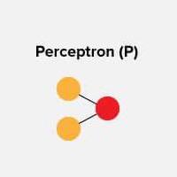
The simplest and oldest model of Neuron, as we know it. A multilayer perceptron has three or more layers. It is used to classify data that cannot be separated linearly. It is a type of artificial neural network that is fully connected. This is because every single node in a layer is connected to each node in the following layer. Inputs are multiplied with weights and fed to the activation function and in backpropagation, they are modified to reduce the loss. In simple words, weights are machine learnt values from Neural Networks. They are depending on the difference between predicted outputs vs training inputs. Nonlinear activation functions are used as an output layer activation function. A multilayer perceptron uses a nonlinear activation function (mainly hyperbolic tangent or logistic function).
Advantages:
- Easy to setup and train
Drawbacks:
- Can only represent a limited set of functions
- Decision boundaries must be hyperplanes
- Can only perfectly separate linearly separable data
Applications:
- Classification
- Encode Database
- Monitor Access Data
2. Deep Convolutional Network (DCN):
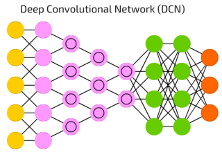
A convolutional neural network uses a variation of the multilayer perceptrons. A CNN contains one or more than one convolutional layers. These layers can either be completely interconnected or pooled. The first layer is called a convolutional layer. Each neuron in the convolutional layer only processes the information from a small part of the visual field. Filters are used to extract certain parts of the image.
Before passing the result to the next layer, the convolutional layer uses a convolutional operation on the input. Due to this convolutional operation, the network can be much deeper but with much fewer parameters. In MLP the inputs are multiplied with weights and fed to the activation function. Convolution uses RELU and MLP uses nonlinear activation function followed by softmax.
Advantages:
- They are flexible and work well on image data
- Have potential for the model to learn useful features from raw data
- They extract informative features from images, eliminating the need of traditional manual image processing methods
Drawbacks:
- They do not encode the position and orientation of object
- Lack of ability to be spatially invariant to the input data
Applications:
- Image and video recognition
- Semantic parsing
- Paraphrase detection
- Anomaly Detection
- NLP
3. Feed-forward (FF):
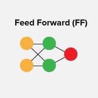
This is form of neural networks where input data moves in one direction only, passing through neural nodes and exiting through output nodes. The hidden layers may or may not be present, input and output layers are present there. They can be further classified as a single-layered or multi-layered feed-forward neural network. This is one of the simplest types of artificial neural networks. In a feedforward neural network, the data passes through the different input nodes until it reaches the output node.
In other words, data moves in only one direction from the first tier onwards until it reaches the output node. This is also known as a front propagated wave which is usually achieved by using a classifying activation function. Number of layers depends on the complexity of the function. It has one-directional forward propagation but no backward propagation.
In this type weights are static. An activation function is fed by inputs which are multiplied by weights. Here we can use classifying activation function or step activation function. For example: The neuron is activated if it is above 0 and the neuron produces 1 as an output. The neuron is not activated if it is below 0 which is considered as -1. They are fairly simple to maintain and are equipped with to deal with data which contains a lot of noise. Unlike in more complex types of neural networks, there is no backpropagation and data moves in one direction only. A feedforward neural network may have as a single layer as well as hidden layers.
In a feedforward neural network, the sum of the products of the inputs and their weights are calculated. This is then fed to the output. Here is an example of a single layer feedforward neural network.
Advantages:
- Computation Speed is very high, as a result of the parallel structure
- Ability to generalize to situations not taught to network previously
- Can be taught to compensate for system changes from initial training model (on-line)
- If an explicit mathematical model is not required, then the network can be programmed in a fraction of the time required for traditional development
Drawbacks:
- The disturbance variables must be measured on-line
- To make effective use of feedforward control, at least an approximate process model should be available
- The quality of feedforward control depends on the accuracy of the process model
- Ideal feedforward controllers that are theoretically capable of achieving perfect control may not be physically realizable
Applications:
- Speech Recognition
- Handwritten Characters Recognition
- Data Compression
- Pattern Recognition
4. Deep Feed-forward (DFF):
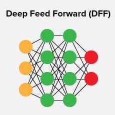
A deep feedforward neural network is an artificial neural network wherein connections between the nodes do not form a cycle. As such, it is different from its descendant: recurrent neural networks.
The feedforward neural network was the first and simplest type of artificial neural network devised. The information moves in only one direction—forward—from the input nodes, through the hidden nodes (if any) and to the output nodes. There are no cycles or loops in the network.
Advantages:
- Easy to learn using optimization algorithms
- Work well in practice
- Deeper networks (with multiple hidden layers) can work better than a single-hidden-layer networks is an empirical observation, despite the fact that their representational power is equal
Drawbacks:
- Deeper networks are more difficult to train
Applications:
- Data Compression
- Financial Prediction
- Pattern Recognition
5. Deconvolutional Neural Networks (DN):
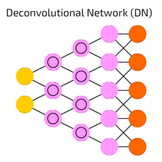
A deconvolutional neural network is a neural network that performs an inverse convolution model. Deconvolutional neural network construct layers from an image in an upward direction.
Deconvolutional neural networks are also known as deconvolutional networks, deconvs or transposed convolutional neural networks. Generally, the DNN involves mapping matrices of pixel values and running a feature selector or other tool over an image. All of this serves the purpose of training machine learning programs, particularly in image processing and computer vision.
Advantages:
- Explaining checkerboard artifacts becomes easy
Drawbacks:
- It usually involves adding many columns and rows of zeros to the input, resulting in a much less efficient implementation
Applications:
- Image resolution
- Optical flow estimation
- Surface depth estimation from an image
6. Deep Convolutional Inverse Graphics Network (DC-IGN):
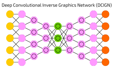
The deep convolutional inverse graphics network (DCIGN) has a model that includes an encoder and a decoder – it is a type of neural network that uses various layers to process input to output results. The encoder consists of several layers of convolutions followed by maxpooling and the decoder has several layers of unpooling (upsampling using nearest neighbors) followed by convolution.
A typical feedforward neural network includes an input layer, hidden layers and output layer. The deep convolutional inverse graphics network uses initial layers to encode through various convolutions, utilizing max pooling, and then uses subsequent layers to decode with unpooling.
The DCIGN also allows the model to understand highly complex concepts such as light intensity, angle and 3D rotation of objects. It will be able to add pictures together, subtract features from an image, understand and perform advanced image operations. For example, the network can identify the features of a dog head and the body of a bird, then combine these features. This is because the DCIGN structure uses the CNN as a data encoder, then the DNN as a decoder.
There are massive implications from this possibility, as what the model can achieve is impressive. For starters, this network is able to perform automatic semantic image segmentation, since the model can detect features within the image, it can accurately extract, mask and track the object of interest in an image and also produce it for us to visually analyze.
Advantages:
- Network can work up a dynamic rendering engine based on aspects like angle and shade
- More intelligent ability to manipulate sophisticated three-dimensional images
Drawbacks:
- Training process takes a lot of time if the computer doesn’t consist of a good GPU
- Requires a large Dataset to process and train the neural network
- Network is significantly slower due to an operation such as maxpool
Applications:
- Manipulation of human faces
7. Hopfield Network (HN):
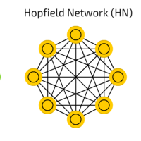
The Hopfield network is an RNN in which all connections are symmetric. It guarantees that it will converge. If the connections are trained using Hebbian learning the Hopfield network can perform as robust content-addressable memory, resistant to connection alteration. Recurrent networks of non-linear units are generally very hard to analyze. They can behave in many different ways: settle to a stable state, oscillate, or follow chaotic trajectories that cannot be predicted far into the future.
A Hopfield network is a network where every neuron is connected to every other neuron. Each node is input before training, then hidden during training and output afterwards. The networks are trained by setting the value of the neurons to the desired pattern after which the weights can be computed. The weights do not change after this.
Once trained for one or more patterns, the network will always converge to one of the learned patterns because the network is only stable in those states.There is another computational role for Hopfield nets. Instead of using the net to store memories, we use it to construct interpretations of sensory input. The input is represented by the visible units, the interpretation is represented by the states of the hidden units, and the badness of the interpretation is represented by the energy.
One of the problem of Hopfield net that it is very limited in its capacity. A Hopfield net of N units can only memorize 0.15N patterns because of the spurious minima in its energy function.
Advantages:
- Simple prescription for the weights, with no training needed
- Output settles down to a steady state
Drawbacks:
- It can rest in a local minimum state instead of a global minimum energy state
- It is very limited in its capacity
Applications:
- Image Detection And Recognition
- Enhancing X-Ray Images
- Optimization Problems
8. Boltzmann Machine (BM):

Boltzmann Machine is a type of stochastic recurrent neural network. It can be interpreted as the stochastic, generative counterpart of Hopfield nets. It was one of the first neural networks capable to represent and solve difficult combinatoric problems. The input neurons become output neurons at the end of a full network update. It starts with random weights and learns through back-propagation. Compared to a Hopfield Net, the neurons mostly have binary activation patterns.
The goal of learning for Boltzmann machine learning algorithm is to maximize the product of the probabilities that the Boltzmann machine assigns to the binary vectors in the training set. This is equivalent to maximizing the sum of the log probabilities that the Boltzmann machine assigns to the training vectors.
In a general Boltzmann machine, the stochastic updates of units need to be sequential. There is a special architecture that allows alternating parallel updates which are much more efficient (no connections within a layer, no skip-layer connections). This mini-batch procedure makes the updates of the Boltzmann machine more parallel. This is called a Deep Boltzmann Machine, a general Boltzmann machine with a lot of missing connections.
Advantages:
- The superiority of the proposed algorithm in the accuracy of recognizing LP rather than other traditional LPRS
Drawbacks:
- Boltzmann learning is significantly slower than backpropagation
- Unrecognized or miss-detected items
Applications:
- Classification
- Regression
- Feature Learning
- Dimensionality Reduction
9. Restricted Boltzmann Machine (RBM):
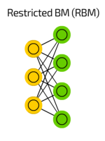
Restricted Boltzmann machine is a generative stochastic artificial neural network that can learn a probability distribution over its set of inputs. As stated earlier, they are a two-layered neural network (one being the visible layer and the other one being the hidden layer) and these two layers are connected by a fully bipartite graph. This means that every node in the visible layer is connected to every node in the hidden layer but no two nodes in the same group are connected to each other. This restriction allows for more efficient training algorithms than what is available for the general class of Boltzmann machines, in particular, the gradient-based contrastive divergence algorithm.
Advantages:
- Find missing values by Gibb’s sampling which is applied to cover the unknown values
- Able to solve imbalanced data problem by SMOTE procedure
- Overcomes the problem of noisy labels by uncorrected label data and its reconstruction errors
Drawbacks:
- Tricky to train well since the common algorithm used
Applications:
- Classification
- Topic modeling
- Collaborative filtering
- Feature learning
- Regression
10. Radial Basis Network (RBN):
Radial Basis Function Network consists of an input vector followed by a layer of RBF neurons and an output layer with one node per category. Classification is performed by measuring the input’s similarity to data points from the training set where each neuron stores a prototype. This will be one of the examples from the training set.
When a new input vector - the n-dimensional vector that you are trying to classify - needs to be classified, each neuron calculates the Euclidean distance between the input and its prototype. For example, if we have two classes i.e. class A and Class B, then the new input to be classified is more close to class A prototypes than the class B prototypes. Hence, it could be tagged or classified as class A.
Each neuron compares the input vector to its prototype and outputs a value ranging which is a measure of similarity from 0 to 1. As the input equals to the prototype, the output of that RBF neuron will be 1 and with the distance grows between the input and prototype the response falls off exponentially towards 0. The curve generated out of neuron’s response tends towards a typical bell curve. The output layer consists of a set of neurons.
A radial basis function considers the distance of any point relative to the centre. Such neural networks have two layers. In the inner layer, the features are combined with the radial basis function.
Then the output of these features is taken into account when calculating the same output in the next time-step. Here is a diagram which represents a radial basis function neural network.
The radial basis function neural network is applied extensively in power restoration systems. In recent decades, power systems have become bigger and more complex.
This increases the risk of a blackout. This neural network is used in the power restoration systems in order to restore power in the shortest possible time.
Advantages:
- In Comparison to MultiLayer Perceptron the training phase is faster as there is no back propagation learning involved
- The interpretation roles of Hidden layer nodes are easy as in comparison to multi layer perceptron
- Number of hidden layer and number of nodes in hidden layer can be choisen but in multi layer perceptron there is no analytical approach to decide the number of nodes in hidden layer or number of hidden layers
Drawbacks:
- Classification is slow in comparison to Multi layer Perceptron due to fact that every node in hidden layer have to compute the RBF function for the input sample vector during classification
Applications:
- Classification
- Function Approximation
- Timeseries Prediction
- System Control
11. Recurrent Neural Network (RNN):

A Recurrent Neural Network is a type of artificial neural network in which the output of a particular layer is saved and fed back to the input. This helps predict the outcome of the layer. Designed to save the output of a layer, Recurrent Neural Network is fed back to the input to help in predicting the outcome of the layer. The first layer is typically a feed forward neural network followed by recurrent neural network layer where some information it had in the previous time-step is remembered by a memory function. Forward propagation is implemented in this case. It stores information required for it’s future use. If the prediction is wrong, the learning rate is employed to make small changes. Hence, making it gradually increase towards making the right prediction during the backpropagation.
The first layer is formed in the same way as it is in the feedforward network. That is, with the product of the sum of the weights and features. However, in subsequent layers, the recurrent neural network process begins. From each time-step to the next, each node will remember some information that it had in the previous time-step. In other words, each node acts as a memory cell while computing and carrying out operations. The neural network begins with the front propagation as usual but remembers the information it may need to use later.
If the prediction is wrong, the system self-learns and works towards making the right prediction during the backpropagation. This type of neural network is very effective in text-to-speech conversion technology. Here’s what a recurrent neural network looks like.
Advantages:
- Can process inputs of any length
- Model is modeled to remember each information throughout the time which is very helpful in any time series predictor
- Even if the input size is larger, the model size does not increase
- The weights can be shared across the time steps
- Can use their internal memory for processing the arbitrary series of inputs which is not the case with feedforward neural networks
Drawbacks:
- Due to its recurrent nature, the computation is slow
- Training of RNN models can be difficult
- If we are using relu or tanh as activation functions, it becomes very difficult to process sequences that are very long
- Prone to problems such as exploding and gradient vanishing
Applications:
- Robot Control
- Speech Recognition
- Time Series Anomaly Detection
- Rhythm Learning
- Music Composition
- Machine Translation
12. Long / Short Term Memory (LSTM):
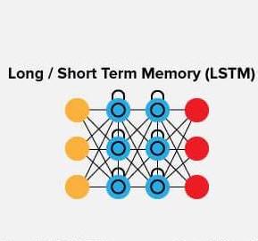
Long Short Term Memory is a special type of (RNN) architecture designed to model long-range dependencies with a higher accuracy in relation to regular. It can be claimed that LSTM is the most successful type of architecture regarding RNN for many tasks with data sequence.
LSTM and regular RNN are usually applied in different task sequence prediction and tagging sequences. Learning data storage through Back propagation Recurrent is time consuming due to insufficient errors in back propagation and deterioration feedback. LSTM is able to learn in a shorter time. In comparison with other neural networks, LSTM is able to act faster with higher accuracy and solve the complex and artificial tasks regarding time delay, something not happened before through none of the recurrent network algorithms.
Many attempts are made to improve LSTM. One recommendation is to apply working memory in LSTM, which would allow the memory cells in different blocks to correspond and the internal computations to be made in one layer of the memory. LSTM avoids the vanishing gradient problem. It works even when with long delays between inputs and can handle signals that mix low and high frequency components. LSTM RNN outperformed other RNN and other sequence learning methods such as HMM in applications such as language learning and connected handwriting recognition. LSTMs networks try to combat the vanishing / exploding gradient problem by introducing gates and an explicitly defined memory cell. The memory cell stores the previous values and holds onto it unless a “forget gate” tells the cell to forget those values. LSTMs also have a “input gate” which adds new stuff to the cell and an “output gate” which decides when to pass along the vectors from the cell to the next hidden state.
Recall that with all RNNs, the values coming in from X_train and H_previous are used to determine what happens in the current hidden state. And the results of the current hidden state (H_current) are used to determine what happens in the next hidden state. LSTMs simply add a cell layer to make sure the transfer of hidden state information from one iteration to the next is reasonably high. Put another way, we want to remember stuff from previous iterations for as long as needed, and the cells in LSTMs allow this to happen. LSTMs have been shown to be able to learn complex sequences, such as writing like Shakespeare or composing primitive music.
LSTMs became popular because they could solve the problem of vanishing gradients. But it turns out, they fail to remove it completely. The problem lies in the fact that the data still has to move from cell to cell for its evaluation. Moreover, the cell has become quite complex now with the additional features (such as forget gates) being brought into the picture. They require a lot of resources and time to get trained and become ready for real-world applications. In technical terms, they need high memory-bandwidth because of linear layers present in each cell which the system usually fails to provide for. Thus, hardware-wise, LSTMs become quite inefficient. With the rise of data mining, developers are looking for a model that can remember past information for a longer time than LSTMs. The source of inspiration for such kind of model is the human habit of dividing a given piece of information into small parts for easy remembrance. LSTMs get affected by different random weight initializations and hence behave quite similar to that of a feed-forward neural net. They prefer small weight initializations instead. LSTMs are prone to overfitting and it is difficult to apply the dropout algorithm to curb this issue. Dropout is a regularization method where input and recurrent connections to LSTM units are probabilistically excluded from activation and weight updates while training a network.
Advantages:
- Advantage in dynamic predicting
- Capturing temporal information
Drawbacks:
- Cannot be trained in parallel
- Transfer learning doesn’t work quite well on LSTMs
Applications:
- Language modelling or text generation
- Image processing
- Speech and Handwriting Recognition
- Music generation
- Language Translation
13. Gated Recurrent Unit (GRU):
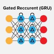
Gated recurrent units are a gating mechanism in recurrent neural networks. The GRU is like a long short-term memory (LSTM) with a forget gate, but has fewer parameters than LSTM, as it lacks an output gate. GRU's performance on certain tasks of polyphonic music modeling, speech signal modeling and natural language processing was found to be similar to that of LSTM. GRUs have been shown to exhibit better performance on certain smaller and less frequent datasets.
Gated recurrent units (GRUs) are a slight variation on LSTMs. They take X_train and H_previous as inputs. They perform some calculations and then pass along H_current. In the next iteration X_train.next and H_current are used for more calculations, and so on. What makes them different from LSTMs is that GRUs don’t need the cell layer to pass values along.
The calculations within each iteration insure that the H_current values being passed along either retain a high amount of old information or are jump-started with a high amount of new information.As mentioned, the Gated Recurrent Units (GRU) is one of the popular variants of recurrent neural networks and has been widely used in the context of machine translation. GRUs can also be regarded as a simpler version of LSTMs (Long Short-Term Memory). The GRU unit was introduced in 2014 and is claimed to be motivated by the Long Short-Term Memory unit. However, the former is much simpler to compute and implement in models.
In most cases, GRUs function very similarly to LSTMs, with the biggest difference being that GRUs are slightly faster and easier to run (but also slightly less expressive). In practice these tend to cancel each other out, as you need a bigger network to regain some expressiveness which then in turn cancels out the performance benefits.
In GRU, two gates including a reset gate that adjusts the incorporation of new input with the previous memory and an update gate that controls the preservation of the precious memory are introduced. The reset gate and the update gate adaptively control how much each hidden unit remembers or forgets while reading/generating a sequence.
Advantages:
- Improve the memory capacity of a recurrent neural network
- Provide the ease of training a model
- Hidden unit can also be used for settling the vanishing gradient problem
- Provide the ease of training a model
Drawbacks:
- Slow convergence
- Low learning efficiency
Applications:
- Speech signal modelling
- Machine translation
- Handwriting recognition
- Natural Language Processing
- Polyphonic Music Modeling
14. Auto Encoder (AE):

An autoencoder is an artificial neural network used to learn efficient data codings in an unsupervised manner. The goal of an autoencoder is to: learn a representation for a set of data, usually for dimensionality reduction by training the network to ignore signal noise. Along with the reduction side, a reconstructing side is also learned, where the autoencoder tries to generate from the reduced encoding a representation as close as possible to its original input. This helps autoencoders to learn important features present in the data.
When a representation allows a good reconstruction of its input then it has retained much of the information present in the input. Recently, the autoencoder concept has become more widely used for learning generative models of data. Autoencoders are neural networks designed for unsupervised learning, i.e. when the data is not labeled.
As a data-compression model, they can be used to encode a given input into a representation of smaller dimension. A decoder can then be used to reconstruct the input back from the encoded version. Autoencoders can use non-linear transformations to encode the given vector into smaller dimensions (as compared to PCA which is a linear transformation). So it can generate more complex encodings.
Advantages:
- They provide flexible mappings
- Learning time is linear (or better) in the number of training cases
- Final encoding model is fairly compact and fast
Drawbacks:
- Difficult to optimize deep auto encoders using back propagation
- With small initial weights, the back propagated gradient dies
Applications:
- Data codings
- Clustering
- Feature Compression
- Classification
15. Variational Autoencoder (VAE):
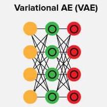
Variational autoencoder models make strong assumptions concerning the distribution of latent variables. They use a variational approach for latent representation learning, which results in an additional loss component and a specific estimator for the training algorithm called the Stochastic Gradient Variational Bayes estimator. It assumes that the data is generated by a directed graphical model and that the encoder is learning an approximation to the posterior distribution where Ф and θ denote the parameters of the encoder (recognition model) and decoder (generative model) respectively. The probability distribution of the latent vector of a variational autoencoder typically matches that of the training data much closer than a standard autoencoder.
Advantages:
- It gives significant control over how we want to model our latent distribution unlike the other models
- After training you can just sample from the distribution followed by decoding and generating new data
Drawbacks:
- Sampling process requires some extra attention
- There is a need to calculate the relationship of each parameter in the network with respect to the final output loss using a technique known as backpropagation
Applications:
- Automatic Image Generation
- Interpolate Between Sentences
16. Denoising Autoencoder (DAE):
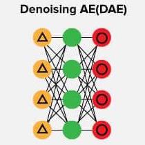
Denoising autoencoders create a corrupted copy of the input by introducing some noise. This helps to avoid the autoencoders to copy the input to the output without learning features about the data. These autoencoders take a partially corrupted input while training to recover the original undistorted input. The model learns a vector field for mapping the input data towards a lower dimensional manifold which describes the natural data to cancel out the added noise.
Advantages:
- It was introduced to achieve good representation
- Corruption of the input can be done randomly by making some of the input as zero
- Minimizes the loss function between the output node and the corrupted input
- Setting up a single-thread denoising autoencoder is easy
Drawbacks:
- To train an autoencoder to denoise data, it is necessary to perform preliminary stochastic mapping in order to corrupt the data and use as input
- This model isn't able to develop a mapping which memorizes the training data because our input and target output are no longer the same
Applications:
- Feature Extraction
- Dimensionality Reduction
17. Sparse Autoencoder (SAE):
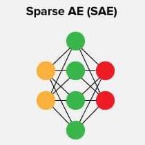
Sparse Autoencoder is a type of autoencoder that employs sparsity to achieve an information bottleneck. Specifically the loss function is constructed so that activations are penalized within a layer. The sparsity constraint can be imposed with L1 regularization or a KL divergence between expected average neuron activation to an ideal distribution
Sparse autoencoders have hidden nodes greater than input nodes. They can still discover important features from the data. A generic sparse autoencoder is visualized where the obscurity of a node corresponds with the level of activation. Sparsity constraint is introduced on the hidden layer. This is to prevent output layer copy input data.
Sparsity may be obtained by additional terms in the loss function during the training process, either by comparing the probability distribution of the hidden unit activations with some low desired value,or by manually zeroing all but the strongest hidden unit activations. Some of the most powerful AIs in the 2010s involved sparse autoencoders stacked inside of deep neural networks.
From the structural point of view, the autoencoder is an axisymmetric single hidden-layer neural network. The autoencoder encodes the input sensor data by using the hidden layer, approximates the minimum error, and obtains the best-feature hidden-layer expression. The concept of the autoencoder comes from the unsupervised computational simulation of human perceptual learning, which itself has some functional flaws. For example, the autoencoder does not learn any practical feature through copying and inputting memory into implicit layers, although it can reconstruct input data with high precision. The sparse autoencoder inherits the idea of the autoencoder and introduces the sparse penalty term, adding constraints to feature learning for a concise expression of the input data.
Advantages:
- Sparsity penalty is applied on the hidden layer in addition to the reconstruction error. This prevents overfitting
- They take the highest activation values in the hidden layer and zero out the rest of the hidden nodes. This prevents autoencoders to use all of the hidden nodes at a time and forcing only a reduced number of hidden nodes to be used
Drawbacks:
- Feature learning requires only unlabeled measurement data
- It's essential that the individual nodes of a trained model which activate are data dependent
Applications:
- Automatic zip code recognition
- Speech recognition
- Self-driving cars
- Feature Extraction
- Handwritten digits Recognition
18. Markov Chain (MC):

A Markov chain is a stochastic model describing a sequence of possible events in which the probability of each event depends only on the state attained in the previous event. A countably infinite sequence, in which the chain moves state at discrete time steps, gives a discrete-time Markov chain (DTMC). A continuous-time process is called a continuous-time Markov chain (CTMC). It is named after the Russian mathematician Andrey Markov.
A Markov model is a mathematical model to represent a randomly changing system under the assumption that future states only depend on the current state (Markov property). It is used for predictive modeling or probabilistic forecasting. A simple model is a Markov chain which models a path through a graph across states (vertices) with given transition probabilities on the edges.
Advantages:
- Temporal nonstationary state transition probabilities can be revised by a parameter learning paradigm
Drawbacks:
- State transition probabilities must be known a priori
Applications:
- Studying cruise control systems in motor vehicles
- Queues or lines of customers arriving at an airport
- Currency exchange rates
- Animal population dynamics
- Queuing Theory
- Statistics
19. Deep Belief Network (DBN):
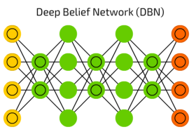
Deep belief network is a generative graphical model, or alternatively a class of deep neural network, composed of multiple layers of latent variables ("hidden units"), with connections between the layers but not between units within each layer.
DBN is a probabilistic, generative model made up of multiple hidden layers. It can be considered a composition of simple learning modules.
DBNs are probabilistic generative models which provide a joint probability distribution over observable data and labels. They are formed by stacking RBMs and training them in a greedy manner.
A DBN initially employs an efficient layer-by-layer greedy learning strategy to initialize the deep network, and, in the sequel, fine-tunes all weights jointly with the desired outputs. DBNs are graphical models which learn to extract a deep hierarchical representation of the training data.
A DBN can be used to generatively pre-train a deep neural network (DNN) by using the learned DBN weights as the initial DNN weights. Various discriminative algorithms can then tune these weights. This is particularly helpful when training data are limited, because poorly initialized weights can significantly hinder learning. These pre-trained weights end up in a region of the weight space that is closer to the optimal weights than random choices. This allows for both improved modeling and faster ultimate convergence.
Back-propagation is considered the standard method in artificial neural networks to calculate the error contribution of each neuron after a batch of data is processed. However, there are some major problems using back-propagation. Firstly, it requires labeled training data; while almost all data is unlabeled. Secondly, the learning time does not scale well, which means it is very slow in networks with multiple hidden layers. Thirdly, it can get stuck in poor local optima, so for deep nets they are far from optimal.
To overcome the limitations of back-propagation, researchers have considered using unsupervised learning approaches. This helps keep the efficiency and simplicity of using a gradient method for adjusting the weights, but also use it for modeling the structure of the sensory input. In particular, they adjust the weights to maximize the probability that a generative model would have generated the sensory input.
Deep Belief Networks can be trained through contrastive divergence or back-propagation and learn to represent the data as a probabilistic model. Once trained or converged to a stable state through unsupervised learning, the model can be used to generate new data. If trained with contrastive divergence, it can even classify existing data because the neurons have been taught to look for different features.
Advantages:
- Fast inference
- Ability to encode richer and higher order network structures
- Greedy layer-by layer learning algorithm can find a good set of model parameters fairly quickly, even for models that contain many layers of nonlinearities and millions of parameters
- Learning algorithm can make efficient use of very large sets of unlabeled data, and so the model can be pre-trained in a completely unsupervised fashion
- There is an efficient way of performing approximate inference to compute the values of the latent variables in the deepest layer, given some input
Drawbacks:
- They do not account for the two-dimensional structure of an input image, which may significantly affect their performance and applicability in computer vision and multimedia analysis problems
- The approximate inference procedure is limited to a single bottom-up pass
- Model can fail to adequately account for uncertainty when interpreting ambiguous sensory inputs
Applications:
- Retrieval of Documents/ Images
- Non-linear Dimensionality Reduction
20. Generative Adversarial Network (GAN):

A generative adversarial network is a class of machine learning frameworks designed by Ian Goodfellow and his colleagues in 2014. Two neural networks contest with each other in a game (in the form of a zero-sum game, where one agent's gain is another agent's loss).
Given a training set, this technique learns to generate new data with the same statistics as the training set. For example, a GAN trained on photographs can generate new photographs that look at least superficially authentic to human observers, having many realistic characteristics. Though originally proposed as a form of generative model for unsupervised learning, GANs have also proven useful for semi-supervised learning, fully supervised learning, and reinforcement learning.
The core idea of a GAN is based on the "indirect" training through the discriminator, which itself is also being updated dynamically. This basically means that the generator is not trained to minimize the distance to a specific image, but rather to fool the discriminator. This enables the model to learn in an unsupervised manner.
In “Generative adversarial nets” (2014), Ian Goodfellow introduced a new breed of neural network, in which 2 networks work together. Generative Adversarial Networks consist of any two networks: one is used for content generating and the other has discriminative function. The discriminative model has the task of determining whether a given image looks natural (an image from the dataset) or looks like it has been artificially created. The task of the generator is to create natural looking images that are similar to the original data distribution. This can be thought of as a zero-sum or minimax two player game. The generator is trying to fool the discriminator while the discriminator is trying to not get fooled by the generator.
Advantages:
- GANs don't require labeled data, they can be trained using unlabeled data as they learn the internal representations of the data
- GANs generate data that is similar to real data
- GANs can learn messy and complicated distributions of data
Drawbacks:
- Training process includes mode collapse, internal covariate shifts, and vanishing gradients
Applications:
- Generate New Human Poses
- Photos to Emojis
- Face Aging
- Super Resolution
- Clothing Translation
- Video games
21. Liquid State Machine (LSM) :
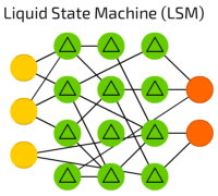
Liquid State Machine is a neural model with real time computations which transforms the time varying inputs stream to a higher dimensional space. The concept of LSM is a novel field of research in biological inspired computation with most research effort on training the model as well as finding the optimum learning method. The performance of LSM model can be investigated using two learning method, online learning and offline (batch) learning methods. The review revealed that optimal performance of LSM was recorded through online method as computational space and other complexities associated with batch learning is eliminated.
LSM is a type of reservoir computer that uses a spiking neural network. An LSM consists of a large collection of units (called nodes, or neurons). Each node receives time varying input from external sources (the inputs) as well as from other nodes. Nodes are randomly connected to each other. The recurrent nature of the connections turns the time varying input into a spatio-temporal pattern of activations in the network nodes. The spatio-temporal patterns of activation are read out by linear discriminant units.
Advantages:
- Continuous time inputs are handled "naturally"
- Computations on various time scales can be done using the same network
- The same network can perform multiple computations
Drawbacks:
- There is no guaranteed way to dissect a working network and figure out how or what computations are being performed
- Very little control over the process.
Applications:
- Speech Recognition
- Computer Vision
22. Extreme Learning Machine (ELM):

Extreme learning machines are feedforward neural networks for classification, regression, clustering, sparse approximation, compression and feature learning with a single layer or multiple layers of hidden nodes, where the parameters of hidden nodes (not just the weights connecting inputs to hidden nodes) need not be tuned. These hidden nodes can be randomly assigned and never updated (i.e. they are random projection but with nonlinear transforms), or can be inherited from their ancestors without being changed. In most cases, the output weights of hidden nodes are usually learned in a single step, which essentially amounts to learning a linear model. The name "extreme learning machine" (ELM) was given to such models by its main inventor Guang-Bin Huang.
In most cases, ELM is used as a single hidden layer feedforward network (SLFN) including but not limited to sigmoid networks, RBF networks, threshold networks, fuzzy inference networks, complex neural networks, wavelet networks, Fourier transform, Laplacian transform, etc. Due to its different learning algorithm implementations for regression, classification, sparse coding, compression, feature learning and clustering, multi ELMs have been used to form multi hidden layer networks, deep learning or hierarchical networks.
Extreme learning machine is a fast growing learning algorithm for the single hidden layer feedforward neural networks used in both classification and regression problems. The ELM used for single hidden layer feedforward neural network training can set the node number of hidden layer and assign the input weights and hidden layer biases randomly, the output layer weights is calculated by the least square method, the entire learning process finished through one mathematical change without the requirement of iteration.
Advantages:
- Short training time
- The number of hidden layer nodes can be randomly selected and analyzed to determine is to reduce the calculation time while learning speed fast
Drawbacks:
- Over-fitting problem
- Decision boundaries must be hyperplanes
- Can only perfectly separate linearly separable data
Applications:
- Data mining
- Artificial intelligence
- Feature Learning
- Clustering
- Regression
23. Echo State Network (ESN):

The echo state network employs a sparsely connected random hidden layer. The weights of output neurons are the only part of the network that are trained. ESN are good at reproducing certain time series.
ESN provide an architecture and supervised learning principle for recurrent neural networks (RNNs). The main idea is (i) to drive a random, large, fixed recurrent neural network with the input signal, thereby inducing in each neuron within this "reservoir" network a nonlinear response signal, and (ii) combine a desired output signal by a trainable linear combination of all of these response signals.
Echo state networks can be set up with or without direct trainable input-to-output connections, with or without output-to-reservoir feedback, with different neuron types, different reservoir-internal connectivity patterns, etc. Furthermore, the output weights can be computed with any of the available offline or online algorithms for linear regression. Besides least-mean-square error solutions (i.e., linear regression weights), margin-maximization criteria known from training support vector machines have been used to determine output weights (Schmidhuber et al. 2007)
The unifying theme throughout all these variations is to use a fixed RNN as a random nonlinear excitable medium, whose high-dimensional dynamical "echo" response to a driving input (and/or output feedback) is used as a non-orthogonal signal basis to reconstruct the desired output by a linear combination, minimizing some error criteria.
ESNs are a novel approach to recurrent neural network training with the advantage of a very simple and linear learning algorithm. It has been demonstrated that ESNs outperform other methods on a number of benchmark tasks. Although the approach is appealing, there are still some inherent limitations in the original formulation. Here we suggest two enhancements of this network model. First, the previously proposed idea of filters in neurons is extended to arbitrary infinite impulse response (IIR) filter neurons. This enables such networks to learn multiple attractors and signals at different timescales, which is especially important for modeling real-world time series. Second, a delay&sum readout is introduced, which adds trainable delays in the synaptic connections of output neurons and therefore vastly improves the memory capacity of echo state networks. It is shown in commonly used benchmark tasks and real-world examples, that this new structure is able to significantly outperform standard ESNs and other state-of-the-art models for nonlinear dynamical system modeling.
Advantages:
- Ability to determine what type of an additional readout is suitable for a task at hand
- Its excellent generalization abilities make it a viable alternative to feed-forward neural networks or relevance-vector-machines
Drawbacks:
- High computational training costs and slow convergence
- Local minima (error function is generally a non convex function)
- Vanishing of the gradient and problem in learning long-term dependencies
Applications:
- Data Mining
- Timeseries Prediction
24. Deep Residual Network (DRN):

Deep Residual Network is an artificial neural network of a kind that builds on constructs known from pyramidal cells in the cerebral cortex. Residual neural networks do this by utilizing skip connections, or shortcuts to jump over some layers. Typical ResNet models are implemented with double- or triple- layer skips that contain nonlinearities (ReLU) and batch normalization in between. An additional weight matrix may be used to learn the skip weights; these models are known as HighwayNets. Models with several parallel skips are referred to as DenseNets. In the context of residual neural networks, a non-residual network may be described as a plain network.
Advantages:
- Can accelerate the speed of training of the deep networks
- Increase depth of the network results in less extra parameters
- Reduce the effect of Vanishing Gradient Problem
- Obtain higher accuracy in network performance especially in Image
Drawbacks:
- In some cases some neuron can “die” in the training and become ineffective/useless. This can cause information loss
- Optimization Difficulty
Applications:
- Image Classification
- Semantic Segmentation
- Speech Recognition
- Language Recognition
25. Kohonen Networks (KN):
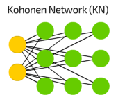
Kohonen Network or self-organizing map (SOM) or self-organizing feature map (SOFM) is a type of artificial neural network (ANN) that is trained using unsupervised learning to produce a low-dimensional (typically two-dimensional), discretized representation of the input space of the training samples, called a map, and is therefore a method to do dimensionality reduction. Self-organizing maps differ from other artificial neural networks as they apply competitive learning as opposed to error-correction learning (such as backpropagation with gradient descent), and in the sense that they use a neighborhood function to preserve the topological properties of the input space.
Both SOM algorithm and SCL algorithm are on-line stochastic algorithms, which means they update the values of the code-vectors (or weight vectors) at each step, that is the arrival or presentation of a new observation. These modifications are instantaneously taken into account through the variations of the distribution and of the statistics along the observed data series. But both algorithms have their deterministic Batch equivalents, which use all the data at each step.
Advantages:
- Simplicity of the computation
- Quickness
- Better final distortion
- No adaptation parameter to tune
- Deterministic reproducible results
Drawbacks:
- Bad organization
- Bad visualization
- Too unbalanced classes
- Strong dependence of the initialization
Applications:
- Project prioritization and selection
- Creation of artwork
- Seismic facies analysis for oil and gas exploration
- Failure mode and effects analysis
26. Support Vector Machines (SVM):
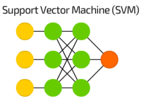
SVM are supervised learning models with associated learning algorithms that analyze data for classification and regression analysis. Given a set of training examples, each marked as belonging to one of two categories, an SVM training algorithm builds a model that assigns new examples to one category or the other, making it a non-probabilistic binary linear classifier.
An SVM maps training examples to points in space so as to maximise the width of the gap between the two categories. New examples are then mapped into that same space and predicted to belong to a category based on which side of the gap they fall.
In addition to performing linear classification, SVMs can efficiently perform a non-linear classification using what is called the kernel trick, implicitly mapping their inputs into high-dimensional feature spaces.
Advantages:
- SVMs deliver a unique solution, since the optimality problem is convex.
- Uses a subset of training points in the decision function (called support vectors), so it is also memory efficient
- Effective in high dimensional spaces
- Versatile: different Kernel functions can be specified for the decision function.
Drawbacks:
- If the number of features is much greater than the number of samples, avoid over-fitting in choosing Kernel functions and regularization term is crucial
- SVMs do not directly provide probability estimates, these are calculated using an expensive five-fold cross-validation
- Lack of transparency of results
Applications:
- Text Categorization
- Face Detection
- Handwriting recognition
27. Neural Turing Machine (NTM):

A Neural Turing Machine is a working memory neural network model. It couples a neural network architecture with external memory resources. The whole architecture is differentiable end-to-end with gradient descent. The models can infer tasks such as copying, sorting and associative recall.
NTM enables agents to store long-term memories by augmenting neural networks with an external memory component. The differentiable architecture of the original NTM can be trained through gradient descent and is able to learn simple algorithms such as copying, sorting and recall from example data. In the work presented here we build on an evolvable version of the NTM (ENTM) that allows the approach to be directly applied to reinforcement learning domains.
NTM architecture contains two basic components: a neural network controller and a memory bank. The Figure presents a high-level diagram of the NTM architecture. Like most neural networks, the controller interacts with the external world via input and output vectors. Unlike a standard network, it also interacts with a memory matrix using selective read and write operations.
NTMs combine the fuzzy pattern matching capabilities of neural networks with the algorithmic power of programmable computers. An NTM has a neural network controller coupled to external memory resources, which it interacts with through attentional mechanisms. The memory interactions are differentiable end-to-end, making it possible to optimize them using gradient descent.[2] An NTM with a long short-term memory (LSTM) network controller can infer simple algorithms such as copying, sorting, and associative recall from examples alone.[1]
Advantages:
- Optimal neural architecture can be learned at the same time
- Hard memory attention mechanism is directly supported and the complete memory does not need to be accessed each time step
- A growing and theoretically infinite memory is possible
Drawbacks:
- As a neural network is trained for a specific task with a fixed number of parameters, it seems impossible for NNs to solve variable-length inputs problems
- RNNs are not good at storing specific information at specific locations
Applications:
- Building an artificial human brain
- Robotics
Conclusions:
There are many types of artificial neural networks that operate in different ways to achieve different outcomes. The most important part about neural networks is that they are designed in a way that is similar to how neurons in the brain work. As a result, they are designed to learn more and improve more with more data and more usage. Unlike traditional machine learning algorithms which tend to stagnate after a certain point, neural networks have the ability to truly grow with more data and more usage.
That’s why many experts believe that different types of neural networks will be the fundamental framework on which next-generation Artificial Intelligence will be built. Hopefully, by now you must have understood the concept of Neural Networks and its types. Moreover, if you are also inspired by the opportunity of Machine Learning, enrol in our Machine Learning and Create your First Application.