Guide for Beginners: Build your First Application
This section describes how to build a simple application using deep learning technique.
A step-by-step complete beginner’s guide to building your first Neural Network in a couple lines of code like a Deep Learning pro!
Writing your first Neural Network can be done with merely a couple lines of code! In this post, we will be exploring how to use Deep Learning for Java to build our first neural network to classify iris flowers. In particular, we will go through the full Deep Learning pipeline, from:
- Exploring and Processing the Data
- Building and Training our Neural Network
- Visualizing Loss and Accuracy
- Evaluate the model's effectiveness
- Use the trained model to make predictions
In just 20 to 30 minutes, you will have coded your own neural network just as a Deep Learning practitioner would have! The only prerequisite is the knowledge of Java. If you have worked with basic Java SE and understand the basic Object-Oriented Programming (OOP) concepts you’ll be good to go. Also, a basic understanding of Neural Network or deep learning and the concepts would be a big plus.
Pre-requisites:
In just 30 minutes, you will have coded your own neural network just as a Deep Learning engineer would have!
Resources you need:
We’ll be using IntelliJ IDEA CE. Download the Community version:
Download IntelliJ IDEA CE
The dataset we will use today is from Kaggle data.
Download Dataset
The Iris classification problem
Imagine you are a botanist seeking an automated way to categorize each Iris flower you find. Machine learning provides many algorithms to classify flowers statistically. For instance, a sophisticated machine learning program could classify flowers based on photographs. We're going to classify Iris flowers based on the length and width measurements of their sepals and petals.
The Iris genus entails about 300 species, but in this guide we will only classify the following three:
- Iris setosa
- Iris virginica
- Iris versicolor
Fortunately, someone has already created a data set of 120 Iris flowers with the sepal and petal measurements. This is a classic dataset that is popular for beginner machine learning classification problems.

Exploring and Processing the Data
Before we code any ML algorithm, the first thing we need to do is to put our data in a format that the algorithm will want. In particular, we need to:
- Read in the CSV (comma separated values) file and convert them to arrays. Arrays are a data format that our algorithm can process.
- Split our dataset into the input features and the label. We’re going to use a CSV version of this data, where columns 0..3 contain the different features of the species and column 4 contains the class of the species, coded with a value 0, 1 or 2.
- Scale the data (we call this normalization) so that the input features have similar orders of magnitude.
- Split our dataset into the training set and the test set.The data is in the form of CSV file. We have a total of 150 records. Out of that, we will choose random 3 for our testing and the rest of the data we will use to train our model.
From this view of the dataset, notice the following:
The first line is a header containing information about the dataset: There are 150 total examples. Each example has four features and one of three possible label names.
Subsequent rows are data records, one example per line, where: The first four fields are features: these are characteristics of an example. Here, the fields hold float numbers representing flower measurements. The last column is the label: this is the value we want to predict. For this dataset, it's an integer value of 0, 1, or 2 that corresponds to a flower name.
Each label is associated with string name (for example, "setosa"), but machine learning typically relies on numeric values. The label numbers are mapped to a named representation, such as:
0: Iris setosa 1: Iris versicolor 2: Iris virginica
Since the dataset is a CSV-formatted text file, Deeplearning4j uses DataVec libraries to read the data from the different sources and convert them to machine-readable format i.e. Numbers. These numbers are called Vectors and the process is called Vectorization.
In this guide we are dealing with CSV, so we will use CSVRecordReader. We will put together a simple utility function that accepts file path, batch size, label index, and a number of classes.

The training data we have for iris flowers are labeled which means the training data is classified into 3 different classes. So we need to tell our CSV reader what column is a label. Also, we need to specify how many total possible classes are there along with batch size to read. We also have to shuffle the training data so that our model could learn more effectively. We will not shuffle of test data as we need to refer them later in the example.
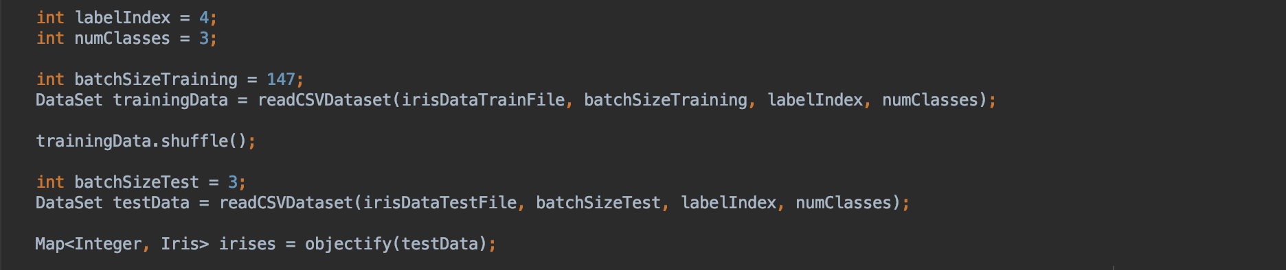
Now let’s write a simple utility method to get our objects. This will read and create an object from your dataset.
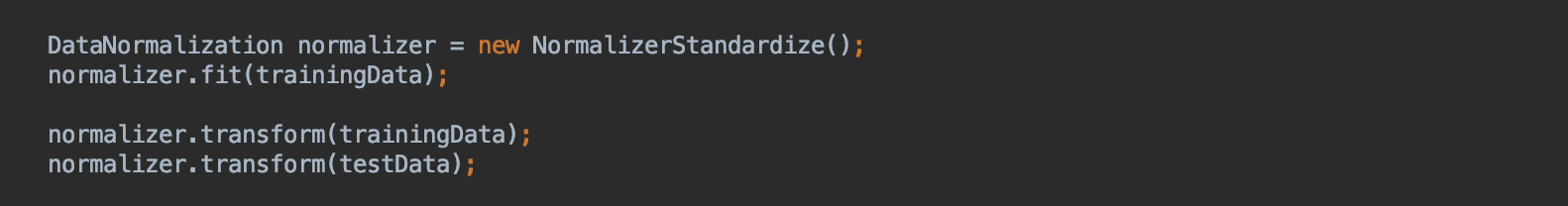
Before building our model we have to normalize our data. This process is called normalization. In Deep Learning, all the data has to be converted to a specific range. either 0,1 or -1,1.
Building and Training our Neural Network
Machine Learning consists of two steps. The first step is to specify an architecture and the second step is to train the model.
First Step: Setting up the Architecture
First we have to select the type of model. A model is a relationship between features and the label. For the Iris classification problem, the model defines the relationship between the sepal and petal measurements and the predicted Iris species. Some simple models can be described with a few lines of algebra, but complex machine learning models have a large number of parameters that are difficult to summarize.

Could you determine the relationship between the four features and the Iris species without using machine learning? Or could you use traditional programming techniques to create a model? Only if you analyzed the dataset long enough to determine the relationships between petal and sepal measurements to a particular species. And this becomes difficult or even impossible on more complicated datasets. A good machine learning approach determines the model for you. If you feed enough representative examples into the right machine learning model type, the program will figure out the relationships for you.
We need to select the model to train. There are many types of models and picking a good one takes experience. This tutorial uses a neural network to solve the Iris classification problem. Neural networks can find complex relationships between features and the label. It is a highly-structured graph, organized into one or more hidden layers. Each hidden layer consists of one or more neurons. There are several categories of neural networks and this program uses a dense, or fully-connected neural network: the neurons in one layer receive input connections from every neuron in the previous layer.
Our model is a linear stack of layers. Its constructor takes a list of layer instances, in this case, two Dense layers with 3 nodes each, and an output layer with 3 nodes representing our label predictions. The first layer's input shape parameter corresponds to the number of features from the dataset, and is required. The activation function determines the output shape of each node in the layer. These non-linearities are important, without them the model would be equivalent to a single layer. There are many available activations, but ReLU is common for hidden layers.
The ideal number of hidden layers and neurons depends on the problem and the dataset. Like many aspects of machine learning, picking the best shape of the neural network requires a mixture of knowledge and experimentation. Increasing the number of hidden layers and neurons typically creates a more powerful model, which requires more data to train effectively.
To make the randomness predictable, we use the concept of seed. The randomness of an artificial neural network(ANN) is when the same neural network is trained on the same data, and it produces different results.
The iterations() method means how many iterations we set to pass through the complete dataset. An iteration is simply one update of the neural net model’s parameters. Not to be confused with an epoch which is one complete pass through the dataset. Many iterations can occur before an epoch is over. Epoch and iteration are only synonymous if you update your parameters once for each pass through the whole dataset; if you update using mini-batches, they mean different things. Say your data has 2 minibatches: A and B. .numIterations(3) performs training like AAABBB, while 3 epochs looks like ABABAB.
The activation() method is a function that runs inside a node to determine its output. The simplest activation function would be linear f(x) = x. To solve complex issues we use non-linear functions. In our case we use ActivationTanH, f(x) = (exp(x) - exp(-x)) / (exp(x) + exp(-x)). At a simple level, activation functions help decide whether a neuron should be activated. This helps determine whether the information that the neuron is receiving is relevant for the input. The activation function is a non-linear transformation that happens over an input signal, and the transformed output is sent to the next neuron.
The weightInit() method specifies weight initialization. Weight initialization refers to the method by which the initial parameters for a new network should be set. Weight initialization are usually defined using the WeightInit enumeration. Correct initial weights affect the results of the training. We set it to a form of Gaussian distribution - WeightInit.XAVIER: with mean 0, variance 2.0/(fanIn + fanOut).
The learningRate() method is used for learning process and affects the ability of the network to learn. The learning rate is one of, if not the most important hyperparameter. If this is too large or too small, your network may learn very poorly, very slowly, or not at all. Typical values for the learning rate are in the range of 0.1 to 1e-6, though the optimal learning rate is usually data (and network architecture) specific. Some simple advice is to start by trying three different learning rates – 1e-1, 1e-3, and 1e-6 – to get a rough idea of what it should be, before further tuning this. Ideally, they run models with different learning rates simultaneously to save time. One of the problems with training neural networks is a case of overfitting when a network “memorizes” the training data. This happens when the network sets excessively high weights for the training data and produces bad results on any other data.
The first layer should contain the same amount of nodes as the columns in the training data. The second dense layer will contain three nodes. This is the value we can variate, but the number of outputs in the previous layer has to be the same. The final output layer should contain the number of nodes matching the number of classes. The structure of the network is shown in the picture. After successful training, we'll have a network that receives four values via its inputs and sends a signal to one of its three outputs. This is a simple classifier.
Finally, to finish building the network, we set up back propagation (one of the most effective training methods) and disable pre-training with the line .backprop(true).pretrain(false).
Second Step: Train the model
Training is the stage of machine learning when the model is gradually optimized, or the model learns the dataset. The goal is to learn enough about the structure of the training dataset to make predictions about unseen data. If you learn too much about the training dataset, then the predictions only work for the data it has seen and will not be generalizable. This problem is called overfitting—it's like memorizing the answers instead of understanding how to solve a problem. The Iris classification problem is an example of supervised machine learning: the model is trained from examples that contain labels. In unsupervised machine learning, the examples don't contain labels. Instead, the model typically finds patterns among the features.
The training model is as easy as calling the fit method on your model. You can also set listeners to log the scores.

Visualizing Loss and Accuracy
We have to define the loss and gradient function. Both training and evaluation stages need to calculate the model's loss. This measures how off a model's predictions are from the desired label, in other words, how bad the model is performing. We want to minimize, or optimize, this value.
Our model will calculate its loss using the the softmax function which takes the model's class probability predictions and the desired label, and returns the average loss across the examples.
An optimizer applies the computed gradients to the model's variables to minimize the loss function. Gradually, the model will find the best combination of weights and bias to minimize loss. And the lower the loss, the better the model's predictions.
The softmax activation function is placed at the output layer of a neural network. It’s commonly used in multi-class learning problems where a set of features can be related to classification. We just have to compute for the normalized exponential function of all the units in the layer. Intuitively, what the softmax does is that it squashes a vector of size K between 0 and 1. Furthermore, because it is a normalization of the exponential, the sum of this whole vector equates to 1 . We can then interpret the output of the softmax as the probabilities that a certain set of features belongs to a certain class.
We can then see that one advantage of using the softmax at the output layer is that it improves the interpretability of the neural network. By looking at the softmax output in terms of the network’s confidence, we can then reason about the behavior of our model. Recall that the softmax function returns probabilities where the whole vector sums to 1. We just take the one with the highest probability then treat it as the network’s prediction.
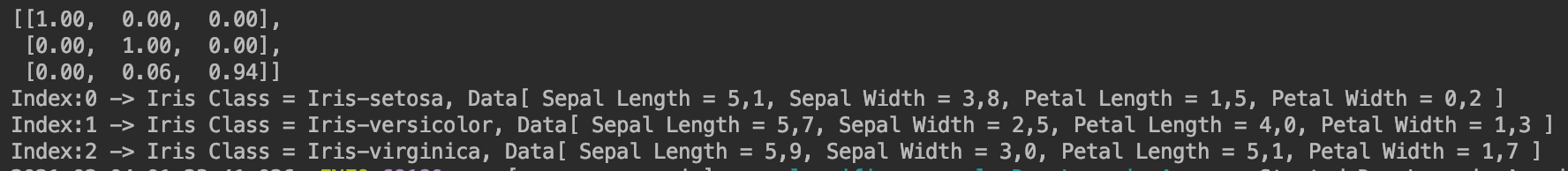
The model does not predict the actual class for you. It only assigns high values to a class which it thinks is more correct. If we look on the output we will see that there could be 3 classes for each of the results. So our model has given us INDArray with some values assigned to in each of the indexes (0,1,2). These indices correspond to classes we defined earlier.
Evaluate the model's effectiveness
Now that the model is trained, we can get some statistics on its performance. Evaluating means determining how effectively the model makes predictions. To determine the model's effectiveness at Iris classification, pass some sepal and petal measurements to the model and ask the model to predict what Iris species they represent. Then compare the model's prediction against the actual label.

Evaluating the model is similar to training the model. The biggest difference is the examples come from a separate test set rather than the training set. To fairly assess a model's effectiveness, the examples used to evaluate a model must be different from the examples used to train the model. The setup for the test Dataset is similar to the setup for training Dataset. For evaluation, you need to provide possible classes that can be one of the outcomes. You get the features (data excluding the labels) from your test data and pass that through your model.

Use the trained model to make predictions
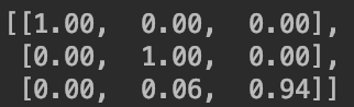
We've trained a model and proven that it's good but not perfect at classifying Iris species. Now let's use the trained model to make some predictions on others examples that contain features but not a label. In real-life, the unlabeled examples could come from lots of different sources including apps, CSV files, and data feeds. For now, we're going to manually provide three unlabeled examples to predict their labels. Recall, the label numbers are mapped to a named representation as: 0: Iris setosa 1: Iris versicolor 2: Iris virginica If we now print out the eval.stats(), we'll see that our network is pretty good at classifying iris flowers, although it did mistake class 1 for class 2 three times.
Conclusion
In this tutorial we go through the steps needed to build your first Neural Network. You just created your first fully functional, application using deap learning!
Download Code